Tournament Style RL: A Stable Reward Signal for Problems With No “Right Answer”

_{📄 Blog post for the paper: “Tournament Style RL: Stabilizing Policy Optimization on Non-Verifiable Problems” — Juneja et al., ICML 2026 (UC Santa Barbara & Google DeepMind). Code: github.com/UCSB-AI/tsrl}

---

TL;DR — For RL on subjective tasks with no ground truth, TSRL rewards each response with its win-rate against a fixed ladder of anchor responses instead of a noisy scalar score. Aggregating $k$ pairwise judgments cuts reward variance by $1/k$ and yields +43.8 points over the base model and +22.8 over the strongest baseline across four tasks.

---

1. Background: Verifiable vs. Non-Verifiable Tasks

1.1 What’s the difference?

	✅ Verifiable tasks	❓ Non-verifiable tasks
Examples	Math problems, code generation, games	Story writing, humor, counseling, tutoring, negotiation
Ground truth?	Yes — an answer key, unit tests, a win/loss condition	No — quality is inherently subjective
Reward for RL	Automatic & exact: correct = 1, wrong = 0	Must be estimated by a human or an LLM judge
Two experts agree?	Always (it’s checkable)	Often not — scores vary significantly across annotators

RL has been spectacularly successful on the left column: Atari, AlphaCode, math reasoning — all powered by rewards computed from an objective correctness signal.

But many of the tasks we care most about live in the right column: mental health support, educational feedback, policy advice, creative writing. There is no answer key — a response isn’t correct, it’s just better or worse than another, and even that judgment is noisy.

1.2 Why is RL on non-verifiable tasks so hard?

The core problem is reward design. If we can’t verify, we must judge — and every existing approach has a failure mode:

Approach	How it works	⚠️ What goes wrong
RLHF / preference learning	Compare two responses; train a reward model	Sparse, noisy, costly; reference moves as the policy improves
Rubric-based scalar scoring	An LLM judge assigns a 0–10 score against a rubric	Scores are coarse and poorly calibrated
Model-internal signals	Use the model’s own confidence / entropy as reward	Can reinforce confidently wrong behavior

The common thread: each sample’s reward is one noisy measurement. That noise hurts in two ways — it flips the ordering between good and bad samples (corrupting the relative advantages GRPO learns from), and it adds variance that destabilizes training.

💡 The key question: Can we build a reward from comparisons (which judges do well) that is also low-variance (many measurements, not one)?

---

2. The Method: Tournament Style RL (TSRL)

2.1 Problem Setting (Paper §2.1)

The notation is minimal:

• A prompt $x$ (e.g., a story premise), and a policy $\pi_\theta(\cdot \mid x)$ that samples a response $c$.
• Every response has a latent quality $q(c) \in \mathbb{R}$ — real but unobservable. The goal is to train $\pi_\theta$ to produce responses with higher $q$.
• A noisy pairwise judge (an LLM) that, given two responses $a, b$, returns a binary verdict:

\[\mathbb{I}[a \succ b] \in \{0, 1\}, \qquad \Pr(a \succ b) = f\big(q(a) - q(b)\big)\]

where $f$ is a strictly increasing bounded function (the Bradley–Terry / Luce comparator model). Verdicts are assumed conditionally independent across anchors.

• For scalar baselines, a rubric scorer is modeled as a single noisy score: $s(c) = q(c) + \varepsilon$, with $\varepsilon \sim \mathcal{N}(0, \sigma_{\text{rub}}^2)$.

2.2 The TSRL Algorithm (Paper §2.2)

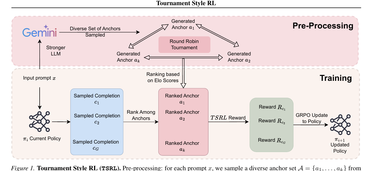
TSRL has two phases:

Phase 1 — Pre-processing (build the ladder, once per prompt):

1. Sample $k$ diverse anchor responses $\mathcal{A} = {r_1, \dots, r_k}$ for each prompt — from a stronger LLM (e.g., Gemini-2.5-Pro) or from human-written references.
2. Run a round-robin tournament among the anchors using a rubric-guided LLM judge, and rank them (Elo-style aggregation / topological sort of the comparison graph).
3. This ranked ladder is frozen — it becomes a stable reference frame for the entire training run.

Phase 2 — Training (every RL step):

1. The current policy $\pi_i$ samples a group of $G$ completions ${c_1, \dots, c_G}$ for a prompt.
2. Each completion $c_j$ is compared against every anchor by the same rubric-guided judge, producing binary outcomes $\mathbb{I}[c_j \succ r_\ell]$.
3. The reward is simply the win-rate:

\[w(c) = \frac{1}{k}\sum_{i=1}^{k} \mathbb{I}[c \succ r_i]\]

1. Plug $w(c)$ into a standard GRPO update (rewards centered by the group mean $b$):

\[\nabla_\theta J \approx \mathbb{E}_{c \sim \pi_\theta}\Big[\big(w(c) - b\big)\, \nabla_\theta \log \pi_\theta(c)\Big]\]

That’s the whole method. No reward model to train, no absolute scores — just “how many anchors did you beat?”

A one-line intuition for why averaging helps. If the judge flips each verdict with probability $e$, a single comparison has variance $e(1-e)$, but the win-rate over $m$ anchors has variance $\frac{e(1-e)}{m}$ — so 8 anchors = 8× less reward noise.

---

3. Why It Works: Three Reward Regimes, Head-to-Head (Paper §2.3–2.4)

Take two candidates where $c_1$ is genuinely better: $q(c_1) > q(c_2)$. For each reward regime, the paper analyzes two quantities: the misordering probability (chance that $c_2$ gets a higher reward — which flips the sign of the GRPO advantage) and the reward variance (which sets the noise level of the gradient).

3.1 Regime ①: TSRL Tournament Reward

Misordering. The win-rate gap $D = w(c_1) - w(c_2)$ is an average of $k$ independent bounded terms with mean $\Delta\mu > 0$, so Hoeffding’s inequality gives

\[\Pr\big(w(c_2) \ge w(c_1)\big) \;\le\; \exp\!\left(-\frac{(\Delta\mu)^2\, k}{2}\right) \;\le\; e^{-ck}\]

— decays exponentially in the number of anchors $k$.

Variance.

\[\mathrm{Var}\big(w(c)\big) = \frac{1}{k^2}\sum_{i=1}^{k} p_i(c)\big(1 - p_i(c)\big) \;\le\; \frac{1}{4k}\]

— shrinks as $1/k$; every extra anchor is another averaged coin flip.

3.2 Regime ②: Single-Pair Comparison (RLHF-style)

Reward = one Bernoulli verdict against one anchor $r$: $S(c) = \mathbb{I}[c \succ r]$, with $p_j = f(q(c_j) - q(r))$.

Misordering.

\[\Pr\big(S(c_2) > S(c_1)\big) = p_2\,(1 - p_1)\]

— a constant that never improves with $k$ and depends entirely on the margin to the one chosen anchor.

Variance.

\[\mathrm{Var}\big(S(c)\big) = p(1-p) \le \frac{1}{4}\]

— $O(1)$, and in real RLHF the comparison partner itself moves as the policy improves, adding even more noise.

3.3 Regime ③: Rubric Scalar Scoring

Reward = one noisy absolute score: $s(c) = q(c) + \varepsilon$, $\varepsilon \sim \mathcal{N}(0, \sigma_{\text{rub}}^2)$.

Misordering.

\[\Pr\big(s(c_1) < s(c_2)\big) = \Phi\!\left(-\frac{\Delta q}{\sqrt{2}\,\sigma_{\text{rub}}}\right)\]

— a constant set by the quality gap and the judge’s calibration.

Variance.

\[\mathrm{Var}\big(s(c)\big) = \sigma_{\text{rub}}^2\]

— an irreducible noise floor per evaluation.

3.4 The Scoreboard

	① TSRL win-rate	② Single pair	③ Rubric scalar
Misordering probability	$\le e^{-ck}$ — decays exponentially with $k$	$p_2(1-p_1)$ — constant	$\Phi!\big(-\tfrac{\Delta q}{\sqrt{2}\sigma_{\text{rub}}}\big)$ — constant
Reward variance	$\le \dfrac{1}{4k}$ — shrinks as $1/k$	$\le \dfrac{1}{4}$ — $O(1)$	$\sigma_{\text{rub}}^2$ — irreducible
Reference frame	Fixed anchor ladder	One (possibly moving) anchor	Ill-calibrated absolute scale

💡 Takeaway 1: Only the tournament reward has an error rate you can drive down by adding anchors — the other two hit a fixed noise floor.

💡 Takeaway 2: Since GRPO learns from centered advantages, cutting reward variance by $1/k$ directly cuts gradient noise — smoother, more sample-efficient training.

---

4. Experimental Setup (Paper §3)

Four non-verifiable tasks, chosen so that quality is genuinely subjective:

Task	Dataset	Anchors from	What makes it non-verifiable
Story generation	WritingPrompts	Human-written completions	Creativity, coherence, style
Constrained humor	MWAHAHA (write a joke using two given words)	Gemini-2.5-Pro (quality spectrum)	Is it funny? Highly subjective
Webpage design	WebSight-Described (text → HTML)	Reference pages	Rendered visual quality judged by a VLM
Mental health counseling	MentalChat16K	Human counselor responses	Many valid answers; helpfulness is subjective

Setup details:

• Backbones: LLaMA-3.1-8B and Qwen-3-4B, full fine-tuning with GRPO (group size $G = 8$, $k = 4$ anchors in the main runs).
• Judge: Kimi-K2 with task-specific rubrics (criteria first, overall quality as tie-break); Kimi-K2-VL judges rendered webpages.
• Evaluation: win-rate (%) against the reference anchors on a held-out test set, mean over 3 runs.

Baselines (all trained under identical optimization settings):

1. Base Model — untrained starting point
2. SFT / Distillation — fine-tune on the top half of the anchor responses
3. Rubrics — RL with a scalar rubric score as reward (Regime ③, the strongest baseline)
4. RLHF (RM) — train a reward model on anchor pairs, then RL (Regime ②)
5. One Anchor — single pairwise comparison vs. the best anchor (Regime ②)
6. Intuitor — intrinsic entropy-based reward (model-internal signal)

⚖️ Fairness note — equal judge budget. TSRL makes $k$ judge calls per sample vs. 1 for the baselines, so the single-comparison baselines are trained for 4× more gradient steps to equalize total judge calls.

---

5. Results (Paper §4)

5.1 Comparison with Existing Techniques (§4.1)

• Setting: TSRL ($k = 4$ anchors) is compared against all six baselines on 4 tasks × 2 backbones, with the single-comparison baselines trained for 4× the gradient steps to equalize the judge budget.
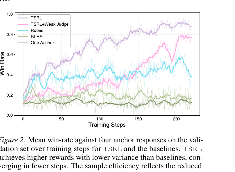
• Result & takeaway: TSRL is best on every task and backbone — +40.0/+40.1 over SFT and +22.6/+22.9 over the rubric baseline (LLaMA / Qwen) — with smoother, more sample-efficient training curves (Figure 2), exactly as the variance-reduction theory predicts.

Table 1 (from the paper). Win-rate (%) vs. the reference anchor set on held-out prompts. Standard deviations in parentheses.

LLaMA-3.1-8B

Method	Stories	Humor	Web	MentalH.
Base Model	13.5 (1.8)	54.0 (2.1)	40.5 (1.4)	30.2 (1.9)
SFT	14.0 (1.5)	56.0 (1.2)	47.2 (2.3)	34.8 (1.7)
One Anchor	13.5 (2.4)	60.0 (1.9)	42.1 (1.6)	32.5 (2.0)
RLHF (RM)	40.5 (1.1)	58.0 (2.2)	54.0 (1.5)	44.7 (1.8)
Rubrics	47.5 (1.3)	62.0 (1.6)	61.2 (2.4)	50.9 (1.2)
Intuitor	14.2 (2.0)	56.4 (1.7)	46.8 (2.1)	34.1 (1.5)
TSRL	74.0 (0.4)	94.0 (0.3)	76.8 (0.5)	67.2 (0.4)
+ Bad Judge	70.0 (0.6)	91.0 (0.5)	71.2 (0.7)	61.5 (0.6)
+ Low Diversity	12.8 (1.5)	55.4 (1.4)	39.1 (2.6)	30.8 (1.5)

Qwen-3-4B

Method	Stories	Humor	Web	MentalH.
Base Model	12.8 (1.6)	52.4 (2.3)	41.2 (1.9)	30.5 (1.4)
SFT	14.5 (1.2)	55.2 (1.8)	48.0 (1.5)	35.1 (2.2)
One Anchor	13.2 (2.1)	58.6 (1.4)	43.5 (2.0)	32.8 (1.7)
RLHF (RM)	39.2 (1.9)	57.5 (2.5)	55.4 (1.3)	45.2 (2.1)
Rubrics	46.1 (1.4)	61.2 (1.1)	62.8 (2.2)	51.7 (1.8)
Intuitor	14.8 (2.3)	54.9 (1.6)	47.5 (1.9)	34.6 (2.0)
TSRL	73.2 (0.5)	93.1 (0.2)	78.5 (0.4)	68.4 (0.5)
+ Bad Judge	68.5 (0.7)	89.2 (0.6)	72.1 (0.8)	62.3 (0.7)
+ Low Diversity	12.1 (2.4)	54.3 (1.5)	40.8 (0.6)	31.2 (1.4)

5.2 Scaling the Number of Anchors (§4.2)

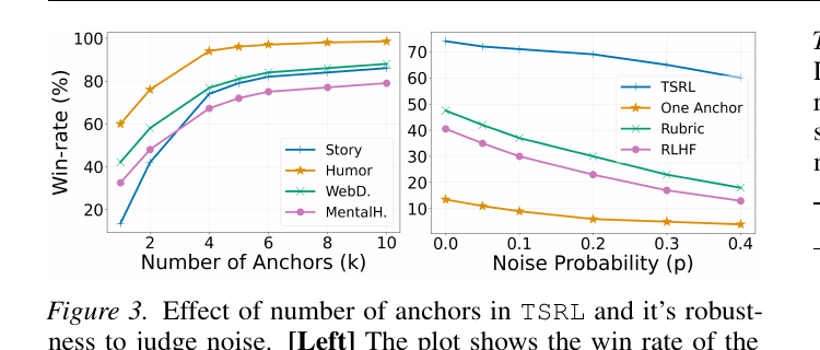
• Setting: Vary the number of anchors $k \in {1, 2, 4, 5, 6, 8, 10}$ while keeping the training data, number of updates, and optimization hyperparameters fixed.
• Result & takeaway: Performance improves by +52 win-rate points on average from $k=1$ to $k=10$, with gains saturating around $k \approx 4$ — the sweet spot given judge cost.

5.3 Effect of Anchor Diversity (§4.3)

• Setting: Train with identical $k$ and compute on two anchor pools — high-diversity (varied styles, from differently-prompted Gemini-2.5-Pro) vs. low-diversity (near-duplicate responses).
• Result & takeaway: High-diversity anchors win by 43.6 points, and low-diversity training collapses to base-model level — anchor diversity is a critical design factor.

5.4 Effect of Judge Noise (§4.4)

• Setting: Replace the strong judge (Kimi-K2) with a much weaker one (LLaMA-3.1-8B), keeping anchors, prompts, and hyperparameters unchanged, and retrain all methods.
• Result & takeaway: TSRL retains ≈94.6% of its performance (−4.2 pts on average) while rubric-based training drops −11.2 pts — you don’t need a frontier-level judge.

Table 2 (from the paper). Win-rate (%) under the weak judge, LLaMA-3.1-8B backbone.

Method (Weak Judge)	Stories	Humor	MentalH.
Base Model	13.5	54.0	30.2
One Anchor	12.0	52.0	30.5
Rubric-based Judge	34.0	51.0	41.8
TSRL	70.0	91.0	61.5

5.5 Artificial Noise Injection (§4.5)

• Setting: Artificially flip each pairwise judgment independently with probability $p \in {0, 0.05, 0.1, 0.2, 0.3, 0.4}$, keeping all other training parameters fixed.
• Result & takeaway: At $p = 0.3$ TSRL retains over 80% of its clean-judge performance while single-pair and scalar-reward methods lose over 40% of their gains (Figure 3, right) — graceful degradation under noise.

5.6 Generalization across Model Scales (§4.6)

• Setting: Repeat story-generation training on two additional policy sizes — Qwen2.5-3B-Instruct and Qwen2.5-7B-Instruct.
• Result & takeaway: TSRL reaches 59.2 (3B) and 78.0 (7B), and the gap over the rubric baseline grows from +14.2 to +28.0 with scale — stronger policies benefit more from a stable reference frame.

5.7 Comparison with Preference Optimization (§4.7)

• Setting: Train LLaMA-3.1-8B with DPO on preference pairs built from the same anchor responses (story generation) — i.e., optimize the same comparisons offline.
• Result & takeaway: DPO reaches 57.5 vs. 74.0 for TSRL — on-policy optimization against a fixed reference ladder beats offline preference optimization over the same comparisons.

5.8 Effect of Anchor Quality (§4.8)

• Setting: Build story-generation anchors from three sources of increasing quality — Gemini-2.5-Flash, Gemini-2.5-Pro, and human writers — and train LLaMA-3.1-8B with each.
• Result & takeaway: Win-rate rises with anchor quality (Flash 65.5 → Pro 70.0 → human 74.0), yet even weak-model anchors far exceed the rubric baseline (47.5) — quality helps but degrades gracefully.

Table 3 (from the paper). Story generation, LLaMA-3.1-8B, by anchor source.

Method	Win Rate
Base model	13.5
Rubrics (strongest baseline)	47.5
TSRL (Gemini-2.5-Flash anchors)	65.5
TSRL (Gemini-2.5-Pro anchors)	70.0
TSRL (human anchors)	74.0

5.9 Disentangling the Stable Reference Frame (§4.9)

• Setting: Add a baseline that ranks the $G = 8$ in-batch completions against each other and rewards the in-batch rank — same aggregation of comparisons, but a moving reference instead of a fixed ladder.
• Result & takeaway: In-batch ranking reaches only 55.0 vs. 74.0 for TSRL — the fixed anchor ladder, not just the extra comparisons, is the main driver of the gains.

5.10 Self-Bootstrapped TSRL without an External Model (§4.10)

• Setting: Sample the anchor set from the policy being trained via four quality-tier prompts (low-effort → top-tier), refreshing anchors every 50 steps — no stronger model or human references involved.
• Result & takeaway: Self-bootstrapped TSRL reaches 81.5, beating external-anchor TSRL (74.0) with no external model at all — anchor refreshing acts as an automatic curriculum that compounds with the stable reference frame.

Table 4 (from the paper). Self-bootstrapped TSRL on story generation (LLaMA-3.1-8B), evaluated against the same held-out human anchors.

Method	Step	Win Rate	Δ vs. base
Base model	0	13.5	—
Self-Bootstrap (Iter 1)	50	40.5	+27.0
Self-Bootstrap (Iter 2)	100	77.5	+64.0
Self-Bootstrap (Iter 3)	150	80.0	+67.5
Self-Bootstrap (Iter 4)	200	81.5	+69.0
TSRL (external anchors)	220	74.0	+60.5
Rubrics	880	47.5	+34.0

5.11 Compute and Judge-Cost Analysis (§4.11)

• Setting: TSRL makes $k$× more judge calls per step ($B \cdot G \cdot T \cdot k$ vs. $B \cdot G \cdot T$), so baselines are run for 4× the gradient steps to compare under a fixed judge budget (comparable judge spend per run).
• Result & takeaway: TSRL at 220 steps (74.0, ~2.5 h) still beats the rubric baseline at 880 steps (47.5, ~7 h) — more efficient per unit of judge compute, not just per gradient step.

5.12 Human Study (§4.12)

• Setting: A blinded study on 50 held-out prompts each for jokes and stories — generations from all methods plus the anchors, randomly ordered, ranked best-to-worst by 6 independent annotators per input (agreement: 0.554 / 0.606).
• Result & takeaway: Humans favor TSRL with 82.9% (jokes) / 84.2% (stories) average win-rates, and LLM-judge rankings correlate strongly with human rankings (Spearman ρ ≈ 0.833, p < 0.01) — the gains reflect real human-perceived quality, not judge artifacts.

---

6. Final Takeaways

Wrapping up — the five things to remember:

1. Comparisons > scores, and many comparisons > one. Judges are unreliable at absolute scoring but usable at pairwise verdicts; averaging $k$ verdicts against a fixed anchor ladder gives a reward whose misordering probability decays as $e^{-ck}$ and whose variance decays as $1/k$ — while single-pair and rubric-scalar rewards are stuck at a constant noise floor.

2. Low-variance rewards = reliable GRPO advantages. Since group-relative methods learn purely from relative rewards within a batch, cutting reward noise directly cuts gradient noise — visible as smoother curves, faster convergence, and tiny run-to-run deviations.

3. It works, broadly. Best method on all 4 non-verifiable tasks × 2 backbones (+43.8 over base, +22.8 over the strongest baseline on average), holds under a fair equal-judge-budget protocol, and is confirmed by blinded human studies.

4. Design rules of thumb: use ~4 diverse anchors (diversity is critical — 43.6-point swing; quality helps but even weak-model anchors work); the judge can be weak (94.6% performance retained); the fixed reference frame contributes more than the extra comparisons do.

5. The road ahead: self-improvement. Anchors sampled from the training policy itself and periodically refreshed already beat external anchors (81.5 vs. 74.0) — pointing toward RL on subjective tasks with no stronger teacher in the loop. Open questions: anchor-refresh schedules, diversity constraints, and safeguards against drift once the policy outgrows its ladder (win-rates saturating at 1 kills the learning signal).

One-sentence summary: When you can’t verify, hold a tournament — a fixed ladder of diverse anchors turns a noisy judge into a stable, low-variance reward that makes RL on subjective tasks actually work.

---

_{All figures, tables, and numerical results in this post are from Juneja et al., “Tournament Style RL: Stabilizing Policy Optimization on Non-Verifiable Problems,” ICML 2026. Math rendering requires a KaTeX/MathJax-enabled markdown viewer (e.g., GitHub, VS Code, Obsidian, most blog engines).}